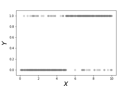
This scatterplot shows the binary $Y$ variables and the corresponding $x$ data for each category.
# #
#
#
#
#
#
#
#
#
#
#
#
#
#
#
#
#
# This shows the fitted logistic regression on the data shown in [Figure](#fig:logreg_001). The points along the curve are the probabilities that each point lies in either of the two categories.
# #
#
#
#
# For a deeper understanding of logistic regression, we need to alter our
# notation slightly and once again use our projection methods. More generally we
# can rewrite Equation ([1](#eq:prob)) as the following,
#
#
#
# $$
# \begin{equation}
# p(\mathbf{x}) = \frac{1}{1+\exp(-\boldsymbol{\beta}^T \mathbf{x})}
# \label{eq:probbeta} \tag{2}
# \end{equation}
# $$
# where $\boldsymbol{\beta}, \mathbf{x}\in \mathbb{R}^n$. From our
# prior work on projection we know that the signed perpendicular distance between
# $\mathbf{x}$ and the linear boundary described by $\boldsymbol{\beta}$ is
# $\boldsymbol{\beta}^T \mathbf{x}/\Vert\boldsymbol{\beta}\Vert$. This means
# that the probability that is assigned to any point in $\mathbb{R}^n$ is a
# function of how close that point is to the linear boundary described by the
# following equation,
# $$
# \boldsymbol{\beta}^T \mathbf{x} = 0
# $$
# But there is something subtle hiding here. Note that
# for any $\alpha\in\mathbb{R}$,
# $$
# \alpha\boldsymbol{\beta}^T \mathbf{x} = 0
# $$
# describes the *same* hyperplane. This means that we can multiply
# $\boldsymbol{\beta}$ by an arbitrary scalar and still get the same geometry.
# However, because of $\exp(-\alpha\boldsymbol{\beta}^T \mathbf{x})$ in Equation
# ([2](#eq:probbeta)), this scaling determines the intensity of the probability
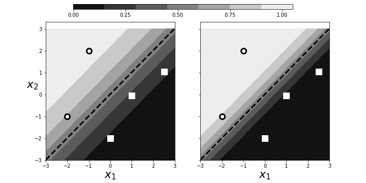
# attributed to $\mathbf{x}$. This is illustrated in [Figure](#fig:logreg_003).
# The panel on the left shows two categories (squares/circles) split by the
# dotted line that is determined by $\boldsymbol{\beta}^T\mathbf{x}=0$. The
# background colors show the probabilities assigned to points in the plane. The
# right panel shows that by scaling with $\alpha$, we can increase the
# probabilities of class membership for the given points, given the exact same
# geometry. The points near the boundary have lower probabilities because they
# could easily be on the opposite side. However, by scaling by $\alpha$, we can
# raise those probabilities to any desired level at the cost of driving the
# points further from the boundary closer to one. Why is this a problem? By
# driving the probabilities arbitrarily using $\alpha$, we can overemphasize the
# training set at the cost of out-of-sample data. That is, we may wind up
# insisting on emphatic class membership of yet unseen points that are close to
# the boundary that otherwise would have more equivocal probabilities (say, near
# $1/2$). Once again, this is another manifestation of bias/variance trade-off.
#
#
#
#
#
#
#
#
#
#
# For a deeper understanding of logistic regression, we need to alter our
# notation slightly and once again use our projection methods. More generally we
# can rewrite Equation ([1](#eq:prob)) as the following,
#
#
#
# $$
# \begin{equation}
# p(\mathbf{x}) = \frac{1}{1+\exp(-\boldsymbol{\beta}^T \mathbf{x})}
# \label{eq:probbeta} \tag{2}
# \end{equation}
# $$
# where $\boldsymbol{\beta}, \mathbf{x}\in \mathbb{R}^n$. From our
# prior work on projection we know that the signed perpendicular distance between
# $\mathbf{x}$ and the linear boundary described by $\boldsymbol{\beta}$ is
# $\boldsymbol{\beta}^T \mathbf{x}/\Vert\boldsymbol{\beta}\Vert$. This means
# that the probability that is assigned to any point in $\mathbb{R}^n$ is a
# function of how close that point is to the linear boundary described by the
# following equation,
# $$
# \boldsymbol{\beta}^T \mathbf{x} = 0
# $$
# But there is something subtle hiding here. Note that
# for any $\alpha\in\mathbb{R}$,
# $$
# \alpha\boldsymbol{\beta}^T \mathbf{x} = 0
# $$
# describes the *same* hyperplane. This means that we can multiply
# $\boldsymbol{\beta}$ by an arbitrary scalar and still get the same geometry.
# However, because of $\exp(-\alpha\boldsymbol{\beta}^T \mathbf{x})$ in Equation
# ([2](#eq:probbeta)), this scaling determines the intensity of the probability
# attributed to $\mathbf{x}$. This is illustrated in [Figure](#fig:logreg_003).
# The panel on the left shows two categories (squares/circles) split by the
# dotted line that is determined by $\boldsymbol{\beta}^T\mathbf{x}=0$. The
# background colors show the probabilities assigned to points in the plane. The
# right panel shows that by scaling with $\alpha$, we can increase the
# probabilities of class membership for the given points, given the exact same
# geometry. The points near the boundary have lower probabilities because they
# could easily be on the opposite side. However, by scaling by $\alpha$, we can
# raise those probabilities to any desired level at the cost of driving the
# points further from the boundary closer to one. Why is this a problem? By
# driving the probabilities arbitrarily using $\alpha$, we can overemphasize the
# training set at the cost of out-of-sample data. That is, we may wind up
# insisting on emphatic class membership of yet unseen points that are close to
# the boundary that otherwise would have more equivocal probabilities (say, near
# $1/2$). Once again, this is another manifestation of bias/variance trade-off.
#
#
#
#
#
# Scaling can arbitrarily increase the probabilities of points near the decision boundary.
# #
#
#
#
# Regularization is a method that controls this effect by penalizing the size of
# $\beta$ as part of its solution. Algorithmically, logistic regression works by
# iteratively solving a sequence of weighted least squares problems. Regression
# adds a $\Vert\boldsymbol{\beta}\Vert/C$ term to the least squares error. To see
# this in action, let's create some data from a logistic regression and see if we
# can recover it using Scikit-learn. Let's start with a scatter of points in the
# two-dimensional plane,
# In[6]:
x0,x1=np.random.rand(2,20)*6-3
X = np.c_[x0,x1,x1*0+1] # stack as columns
# Note that `X` has a third column of all ones. This is a
# trick to allow the corresponding line to be offset from the origin
# in the two-dimensional plane. Next, we create a linear boundary
# and assign the class probabilities according to proximity to the
# boundary.
# In[7]:
beta = np.array([1,-1,1]) # last coordinate for affine offset
prd = X.dot(beta)
probs = 1/(1+np.exp(-prd/np.linalg.norm(beta)))
c = (prd>0) # boolean array class labels
# This establishes the training data. The next block
# creates the logistic regression object and fits the data.
# In[8]:
lr = LogisticRegression()
_=lr.fit(X[:,:-1],c)
# Note that we have to omit the third dimension because of
# how Scikit-learn internally breaks down the components of the
# boundary. The resulting code extracts the corresponding
# $\boldsymbol{\beta}$ from the `LogisticRegression` object.
# In[9]:
betah = np.r_[lr.coef_.flat,lr.intercept_]
# **Programming Tip.**
#
# The Numpy `np.r_` object provides a quick way to stack Numpy
# arrays horizontally instead of using `np.hstack`.
#
#
#
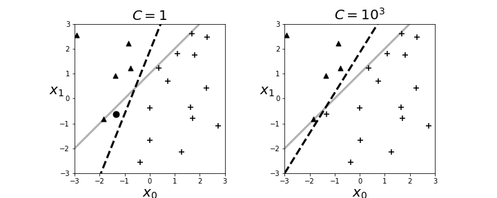
# The resulting boundary is shown in the left panel in [Figure](#fig:logreg_004). The crosses and triangles represent the two classes we
# created above, along with the separating gray line. The logistic regression
# fit produces the dotted black line. The dark circle is the point that logistic
# regression categorizes incorrectly. The regularization parameter is $C=1$ by
# default. Next, we can change the strength of the regularization parameter as in
# the following,
# In[10]:
lr = LogisticRegression(C=1000)
# and the re-fit the data to produce the right panel in
# [Figure](#fig:logreg_004). By increasing the regularization
# parameter, we essentially nudged the fitting algorithm to
# *believe* the data more than the general model. That is, by doing
# this we accepted more variance in exchange for better bias.
#
#
#
#
#
#
#
#
#
#
# Regularization is a method that controls this effect by penalizing the size of
# $\beta$ as part of its solution. Algorithmically, logistic regression works by
# iteratively solving a sequence of weighted least squares problems. Regression
# adds a $\Vert\boldsymbol{\beta}\Vert/C$ term to the least squares error. To see
# this in action, let's create some data from a logistic regression and see if we
# can recover it using Scikit-learn. Let's start with a scatter of points in the
# two-dimensional plane,
# In[6]:
x0,x1=np.random.rand(2,20)*6-3
X = np.c_[x0,x1,x1*0+1] # stack as columns
# Note that `X` has a third column of all ones. This is a
# trick to allow the corresponding line to be offset from the origin
# in the two-dimensional plane. Next, we create a linear boundary
# and assign the class probabilities according to proximity to the
# boundary.
# In[7]:
beta = np.array([1,-1,1]) # last coordinate for affine offset
prd = X.dot(beta)
probs = 1/(1+np.exp(-prd/np.linalg.norm(beta)))
c = (prd>0) # boolean array class labels
# This establishes the training data. The next block
# creates the logistic regression object and fits the data.
# In[8]:
lr = LogisticRegression()
_=lr.fit(X[:,:-1],c)
# Note that we have to omit the third dimension because of
# how Scikit-learn internally breaks down the components of the
# boundary. The resulting code extracts the corresponding
# $\boldsymbol{\beta}$ from the `LogisticRegression` object.
# In[9]:
betah = np.r_[lr.coef_.flat,lr.intercept_]
# **Programming Tip.**
#
# The Numpy `np.r_` object provides a quick way to stack Numpy
# arrays horizontally instead of using `np.hstack`.
#
#
#
# The resulting boundary is shown in the left panel in [Figure](#fig:logreg_004). The crosses and triangles represent the two classes we
# created above, along with the separating gray line. The logistic regression
# fit produces the dotted black line. The dark circle is the point that logistic
# regression categorizes incorrectly. The regularization parameter is $C=1$ by
# default. Next, we can change the strength of the regularization parameter as in
# the following,
# In[10]:
lr = LogisticRegression(C=1000)
# and the re-fit the data to produce the right panel in
# [Figure](#fig:logreg_004). By increasing the regularization
# parameter, we essentially nudged the fitting algorithm to
# *believe* the data more than the general model. That is, by doing
# this we accepted more variance in exchange for better bias.
#
#
#
#
#
# The left panel shows the resulting boundary (dashed line) with $C=1$ as the regularization parameter. The right panel is for $C=1000$. The gray line is the boundary used to assign the class membership for the synthetic data. The dark circle is the point that logistic regression categorizes incorrectly.
# #
#
#
#
#
# ### Maximum Likelihood Estimation for Logistic Regression
#
# Let us again consider the binary classification problem. We define $y_k =
# \mathbb{P}(C_1\vert \mathbf{x}_k)$, the conditional probability of the data as
# a member of given class. Our construction of this problem provides
# $$
# y_k = \theta([\mathbf{w},w_0] \cdot [\mathbf{x}_k,1])
# $$
# where $\theta$ is the logistic function. Recall that there are only
# two classes for this problem. The data set looks like the following,
# $$
# \lbrace(\mathbf{x}_0,r_0),\ldots,(\mathbf{x}_k,r_k),\ldots,(\mathbf{x}_{n-1},r_{n-1})\rbrace
# $$
# where $r_k\in \lbrace 0,1 \rbrace$. For example, we could have the
# following sequence of observed classes,
# $$
# \lbrace C_0,C_1,C_1,C_0,C_1 \rbrace
# $$
# For this case the likelihood is then the following,
# $$
# \ell= \mathbb{P}(C_0\vert\mathbf{x}_0)\mathbb{P}(C_1\vert\mathbf{x}_1)\mathbb{P}(C_1\vert\mathbf{x}_1) \mathbb{P}(C_0\vert\mathbf{x}_0)\mathbb{P}(C_1\vert\mathbf{x}_1)
# $$
# which we can rewrite as the following,
# $$
# \ell(\mathbf{w},w_0)= (1-y_0) y_1 y_2 (1-y_3) y_4
# $$
# Recall that there are two mutually exhaustive classes. More
# generally, this can be written as the following,
# $$
# \ell(\mathbf{w}\vert\mathcal{X})=\prod_k^n y_k^{r_k} (1-y_k)^{1-r_k}
# $$
# Naturally, we want to compute the logarithm of this as the cross-entropy,
# $$
# E = -\sum_k r_k \log(y_k) + (1-r_k)\log(1-y_k)
# $$
# and then minimize this to find $\mathbf{w}$ and $w_0$. This is
# difficult to do with calculus because the derivatives have non-linear terms in
# them that are hard to solve for.
#
# ### Multi-Class Logistic Regression Using Softmax
#
# The logistic regression problem provides a solution for the probability
# between exactly two alternative classes. To extend to the multi-class
# problem, we need the *softmax* function. Consider the likelihood
# ratio between the $i^{th}$ class and the reference class, $\mathcal{C}_k$,
# $$
# \log\frac{p(\mathbf{x}\vert \mathcal{C}_i)}{p(\mathbf{x}\vert\mathcal{C}_k)} = \mathbf{w}_i^T \mathbf{x}
# $$
# Taking the exponential of this and normalizing across all
# the classes gives the softmax function,
# $$
# y_i=p(\mathcal{C}_i \vert\mathbf{x})=\frac{\exp\left(\mathbf{w}_i^T\mathbf{x}\right)}{\sum_k \exp\left( \mathbf{w}_k^T \mathbf{x}\right)}
# $$
# Note that $\sum_i y_i=1$. If the $\mathbf{w}_i^T \mathbf{x}$ term is
# larger than the others, after the exponentiation and normalization, it
# automatically suppresses the other $y_j \forall j \neq i$, which acts like the
# maximum function, except this function is differentiable, hence *soft*, as in
# *softmax*. While that is all straightforward, the trick is deriving the
# $\mathbf{w}_i$ vectors from the training data $\lbrace\mathbf{x}_i,y_i\rbrace$.
#
# Once again, the launching point is the likelihood function. As with the
# two-class logistic regression problem, we have the likelihood as the following,
# $$
# \ell = \prod_k \prod_i (y_i^k)^{r_i^k}
# $$
# The log-likelihood of this is the same as the cross-entropy,
# $$
# E = - \sum_k \sum_i r_i^k \log y_i^k
# $$
# This is the error function we want to minimize. The computation works
# as before with logistic regression, except there are more derivatives to keep
# track of in this case.
#
# ### Understanding Logistic Regression
#
# To generalize this technique beyond logistic regression, we need to re-think
# the problem more abstractly as the data set $\lbrace x_i, y_i \rbrace$. We
# have the $y_i \in \lbrace 0,1 \rbrace$ data modeled as Bernoulli random
# variables. We also have the $x_i$ data associated with each $y_i$, but it is
# not clear how to exploit this association. What we would like is to construct
# $\mathbb{E}(Y|X)$ which we already know (see [ch:prob](#ch:prob)) is the
# best MSE estimator. For this problem, we have
# $$
# \mathbb{E}(Y|X) =\mathbb{P}(Y|X)
# $$
# because only $Y=1$ is nonzero in the summation. Regardless, we
# don't have the conditional probabilities anyway. One way to look at
# logistic regression is as a way to build in the functional relationship
# between $y_i$ and $x_i$. The simplest thing we could do is
# approximate,
# $$
# \mathbb{E}(Y|X) \approx \beta_0 + \beta_1 x := \eta(x)
# $$
# If this is the model, then the target would be the $y_i$ data. We can
# force the output of this linear regression into the interval $[0,1]$ by composing
# it with a sigmoidal function,
# $$
# \theta(x) = \frac{1}{1+\exp(-x)}
# $$
# Then we have a new function $\theta(\eta(x))$ to match against $y_i$ using
# $$
# J(\beta_0,\beta_1) = \sum_i (\theta(\eta(x_i))-y_i)^2
# $$
# This is a nice setup for an optimization problem. We could certainly
# solve this numerically using `scipy.optimize`. Unfortunately, this would take
# us into the black box of the optimization algorithm where we would lose all of
# our intuitions and experience with linear regression. We can take the opposite
# approach. Instead of trying to squash the output of the linear estimator into
# the desired domain, we can map the $y_i$ data into the unbounded space of the
# linear estimator. Thus, we define the inverse of the above $\theta$ function as
# the *link* function.
# $$
# g(y) = \log \left( \frac{y}{1-y} \right)
# $$
# This means that our approximation to the
# unknown conditional expectation is the following,
# $$
# g(\mathbb{E}(Y|X)) \approx \beta_0 + \beta_1 x := \eta(x)
# $$
# We cannot apply this directly to the $y_i$, so we compute the Taylor
# series expansion centered on $\mathbb{E}(Y|X)$, up to the linear term, to obtain the
# following,
# $$
# \begin{align*}
# g(Y) & \approx & g(\mathbb{E}(Y|X)) + (Y-\mathbb{E}(Y|X)) g'(\mathbb{E}(Y|X)) \\
# & \approx & \eta(x) + (Y-\theta(\eta(x))) g'(\theta(\eta(x))) := z
# \end{align*}
# $$
# Because we do not know the conditional expectation, we replaced these
# terms with our earlier $\theta(\eta(x))$ function. This new approximation
# defines our transformed data that we will use to feed the linear model. Note
# that the $\beta$ parameters are embedded in this transformation. The
# $(Y-\theta(\eta(x)))$ term acts as the usual additive noise term. Also,
# $$
# g'(x) = \frac{1}{x(1-x)}
# $$
# The following code applies this transformation to the `xi,yi` data
# In[11]:
import numpy as np
v = 0.9
@np.vectorize
def gen_y(x):
if x<5: return np.random.choice([0,1],p=[v,1-v])
else: return np.random.choice([0,1],p=[1-v,v])
xi = np.sort(np.random.rand(500)*10)
yi = gen_y(xi)
# In[12]:
b0, b1 = -2,0.5
g = lambda x: np.log(x/(1-x))
theta = lambda x: 1/(1+np.exp(-x))
eta = lambda x: b0 + b1*x
theta_ = theta(eta(xi))
z=eta(xi)+(yi-theta_)/(theta_*(1-theta_))
# In[13]:
from matplotlib.pylab import subplots
fig,ax=subplots()
_=ax.plot(xi,z,'k.',alpha=.3)
_=ax2 = ax.twinx()
_=ax2.plot(xi,yi,'.r',alpha=.3)
_=ax2.set_ylabel('Y',fontsize=16,rotation=0,color='r')
_=ax2.spines['right'].set_color('red')
_=ax.set_xlabel('X',fontsize=16)
_=ax.set_ylabel('Z',fontsize=16,rotation=0)
_=ax2.tick_params(axis='y', colors='red')
fig.savefig('fig-machine_learning/glm_001.png')
#
#
#
#
#
#
#
#
#
#
# ### Maximum Likelihood Estimation for Logistic Regression
#
# Let us again consider the binary classification problem. We define $y_k =
# \mathbb{P}(C_1\vert \mathbf{x}_k)$, the conditional probability of the data as
# a member of given class. Our construction of this problem provides
# $$
# y_k = \theta([\mathbf{w},w_0] \cdot [\mathbf{x}_k,1])
# $$
# where $\theta$ is the logistic function. Recall that there are only
# two classes for this problem. The data set looks like the following,
# $$
# \lbrace(\mathbf{x}_0,r_0),\ldots,(\mathbf{x}_k,r_k),\ldots,(\mathbf{x}_{n-1},r_{n-1})\rbrace
# $$
# where $r_k\in \lbrace 0,1 \rbrace$. For example, we could have the
# following sequence of observed classes,
# $$
# \lbrace C_0,C_1,C_1,C_0,C_1 \rbrace
# $$
# For this case the likelihood is then the following,
# $$
# \ell= \mathbb{P}(C_0\vert\mathbf{x}_0)\mathbb{P}(C_1\vert\mathbf{x}_1)\mathbb{P}(C_1\vert\mathbf{x}_1) \mathbb{P}(C_0\vert\mathbf{x}_0)\mathbb{P}(C_1\vert\mathbf{x}_1)
# $$
# which we can rewrite as the following,
# $$
# \ell(\mathbf{w},w_0)= (1-y_0) y_1 y_2 (1-y_3) y_4
# $$
# Recall that there are two mutually exhaustive classes. More
# generally, this can be written as the following,
# $$
# \ell(\mathbf{w}\vert\mathcal{X})=\prod_k^n y_k^{r_k} (1-y_k)^{1-r_k}
# $$
# Naturally, we want to compute the logarithm of this as the cross-entropy,
# $$
# E = -\sum_k r_k \log(y_k) + (1-r_k)\log(1-y_k)
# $$
# and then minimize this to find $\mathbf{w}$ and $w_0$. This is
# difficult to do with calculus because the derivatives have non-linear terms in
# them that are hard to solve for.
#
# ### Multi-Class Logistic Regression Using Softmax
#
# The logistic regression problem provides a solution for the probability
# between exactly two alternative classes. To extend to the multi-class
# problem, we need the *softmax* function. Consider the likelihood
# ratio between the $i^{th}$ class and the reference class, $\mathcal{C}_k$,
# $$
# \log\frac{p(\mathbf{x}\vert \mathcal{C}_i)}{p(\mathbf{x}\vert\mathcal{C}_k)} = \mathbf{w}_i^T \mathbf{x}
# $$
# Taking the exponential of this and normalizing across all
# the classes gives the softmax function,
# $$
# y_i=p(\mathcal{C}_i \vert\mathbf{x})=\frac{\exp\left(\mathbf{w}_i^T\mathbf{x}\right)}{\sum_k \exp\left( \mathbf{w}_k^T \mathbf{x}\right)}
# $$
# Note that $\sum_i y_i=1$. If the $\mathbf{w}_i^T \mathbf{x}$ term is
# larger than the others, after the exponentiation and normalization, it
# automatically suppresses the other $y_j \forall j \neq i$, which acts like the
# maximum function, except this function is differentiable, hence *soft*, as in
# *softmax*. While that is all straightforward, the trick is deriving the
# $\mathbf{w}_i$ vectors from the training data $\lbrace\mathbf{x}_i,y_i\rbrace$.
#
# Once again, the launching point is the likelihood function. As with the
# two-class logistic regression problem, we have the likelihood as the following,
# $$
# \ell = \prod_k \prod_i (y_i^k)^{r_i^k}
# $$
# The log-likelihood of this is the same as the cross-entropy,
# $$
# E = - \sum_k \sum_i r_i^k \log y_i^k
# $$
# This is the error function we want to minimize. The computation works
# as before with logistic regression, except there are more derivatives to keep
# track of in this case.
#
# ### Understanding Logistic Regression
#
# To generalize this technique beyond logistic regression, we need to re-think
# the problem more abstractly as the data set $\lbrace x_i, y_i \rbrace$. We
# have the $y_i \in \lbrace 0,1 \rbrace$ data modeled as Bernoulli random
# variables. We also have the $x_i$ data associated with each $y_i$, but it is
# not clear how to exploit this association. What we would like is to construct
# $\mathbb{E}(Y|X)$ which we already know (see [ch:prob](#ch:prob)) is the
# best MSE estimator. For this problem, we have
# $$
# \mathbb{E}(Y|X) =\mathbb{P}(Y|X)
# $$
# because only $Y=1$ is nonzero in the summation. Regardless, we
# don't have the conditional probabilities anyway. One way to look at
# logistic regression is as a way to build in the functional relationship
# between $y_i$ and $x_i$. The simplest thing we could do is
# approximate,
# $$
# \mathbb{E}(Y|X) \approx \beta_0 + \beta_1 x := \eta(x)
# $$
# If this is the model, then the target would be the $y_i$ data. We can
# force the output of this linear regression into the interval $[0,1]$ by composing
# it with a sigmoidal function,
# $$
# \theta(x) = \frac{1}{1+\exp(-x)}
# $$
# Then we have a new function $\theta(\eta(x))$ to match against $y_i$ using
# $$
# J(\beta_0,\beta_1) = \sum_i (\theta(\eta(x_i))-y_i)^2
# $$
# This is a nice setup for an optimization problem. We could certainly
# solve this numerically using `scipy.optimize`. Unfortunately, this would take
# us into the black box of the optimization algorithm where we would lose all of
# our intuitions and experience with linear regression. We can take the opposite
# approach. Instead of trying to squash the output of the linear estimator into
# the desired domain, we can map the $y_i$ data into the unbounded space of the
# linear estimator. Thus, we define the inverse of the above $\theta$ function as
# the *link* function.
# $$
# g(y) = \log \left( \frac{y}{1-y} \right)
# $$
# This means that our approximation to the
# unknown conditional expectation is the following,
# $$
# g(\mathbb{E}(Y|X)) \approx \beta_0 + \beta_1 x := \eta(x)
# $$
# We cannot apply this directly to the $y_i$, so we compute the Taylor
# series expansion centered on $\mathbb{E}(Y|X)$, up to the linear term, to obtain the
# following,
# $$
# \begin{align*}
# g(Y) & \approx & g(\mathbb{E}(Y|X)) + (Y-\mathbb{E}(Y|X)) g'(\mathbb{E}(Y|X)) \\
# & \approx & \eta(x) + (Y-\theta(\eta(x))) g'(\theta(\eta(x))) := z
# \end{align*}
# $$
# Because we do not know the conditional expectation, we replaced these
# terms with our earlier $\theta(\eta(x))$ function. This new approximation
# defines our transformed data that we will use to feed the linear model. Note
# that the $\beta$ parameters are embedded in this transformation. The
# $(Y-\theta(\eta(x)))$ term acts as the usual additive noise term. Also,
# $$
# g'(x) = \frac{1}{x(1-x)}
# $$
# The following code applies this transformation to the `xi,yi` data
# In[11]:
import numpy as np
v = 0.9
@np.vectorize
def gen_y(x):
if x<5: return np.random.choice([0,1],p=[v,1-v])
else: return np.random.choice([0,1],p=[1-v,v])
xi = np.sort(np.random.rand(500)*10)
yi = gen_y(xi)
# In[12]:
b0, b1 = -2,0.5
g = lambda x: np.log(x/(1-x))
theta = lambda x: 1/(1+np.exp(-x))
eta = lambda x: b0 + b1*x
theta_ = theta(eta(xi))
z=eta(xi)+(yi-theta_)/(theta_*(1-theta_))
# In[13]:
from matplotlib.pylab import subplots
fig,ax=subplots()
_=ax.plot(xi,z,'k.',alpha=.3)
_=ax2 = ax.twinx()
_=ax2.plot(xi,yi,'.r',alpha=.3)
_=ax2.set_ylabel('Y',fontsize=16,rotation=0,color='r')
_=ax2.spines['right'].set_color('red')
_=ax.set_xlabel('X',fontsize=16)
_=ax.set_ylabel('Z',fontsize=16,rotation=0)
_=ax2.tick_params(axis='y', colors='red')
fig.savefig('fig-machine_learning/glm_001.png')
#
#
#
#
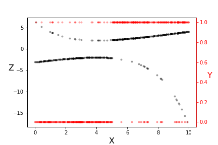
# The transformation underlying logistic regression.
# #
#
#
#
# Note the two vertical scales shown in [Figure](#fig:glm_001). The red scale on the
# right is the $\lbrace 0,1 \rbrace$ domain of the $y_i$ data (red dots) and the
# left scale is transformed $z_i$ data (black dots). Note that the transformed
# data is more linear where the original data is less equivocal at the extremes.
# Also, this transformation used a specific pair of $\beta_i$ parameters. The
# idea is to iterate over this transformation and derive new $\beta_i$
# parameters. With this approach, we have
# $$
# \mathbb{V}(Z|X) = (g')^2 \mathbb{V}(Y|X)
# $$
# Recall that, for this binary variable, we have
# $$
# \mathbb{P}(Y|X) = \theta(\eta(x)))
# $$
# Thus,
# $$
# \mathbb{V}(Y|X) = \theta(\eta(x)) (1-\theta(\eta(x)))
# $$
# from which we obtain
# $$
# \mathbb{V}(Z|X) = \left[ \theta(\eta(x))(1-\theta(\eta(x))) \right]^{-1}
# $$
# The important fact here is the variance is a function of the $X$
# (i.e., heteroskedastic). As we discussed with Gauss-Markov, the appropriate
# linear regression is weighted least-squares where the weights at each data
# point are inversely proportional to the variance. This ensures that the
# regression process accounts for this heteroskedasticity. Numpy has a weighted
# least squares implemented in the `polyfit` function,
# In[14]:
w=(theta_*(1-theta_))
p=np.polyfit(xi,z,1,w=np.sqrt(w))
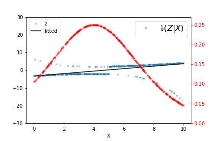
# The output of this fit is shown in [Figure](#fig:glm_002), along
# with the raw data and $\mathbb{V}(Z|X)$ for this particular fitted $\beta_i$.
# Iterating a few more times refines the estimated line but it does not take many
# such iterations to converge. As indicated by the variance line, the fitted line
# favors the data at either extreme.
# In[15]:
fig,ax=subplots()
ax2 = ax.twinx()
theta_ = theta(eta(xi))
_=ax.plot(xi,
z,
'.',alpha=.3,
label='z'
);
_=ax.axis(ymax=30,ymin=-30);
_=ax2.plot(xi,theta_*(1-theta_),'.r',alpha=.3,label='$\mathbb{V}(Z|X)$');
_=ax2.axis(ymax=0.27,ymin=0);
p=np.polyfit(xi,z,1,w=np.sqrt(w));
_=ax.plot(xi,np.polyval(p,xi),'k',label='fitted');
_=ax2.legend(fontsize=16);
_=ax.legend(loc=2);
_=ax.set_xlabel('X');
_=ax2.tick_params(axis='y', colors='red');
fig.savefig('fig-machine_learning/glm_002.png');
#
#
#
#
#
#
#
#
#
# Note the two vertical scales shown in [Figure](#fig:glm_001). The red scale on the
# right is the $\lbrace 0,1 \rbrace$ domain of the $y_i$ data (red dots) and the
# left scale is transformed $z_i$ data (black dots). Note that the transformed
# data is more linear where the original data is less equivocal at the extremes.
# Also, this transformation used a specific pair of $\beta_i$ parameters. The
# idea is to iterate over this transformation and derive new $\beta_i$
# parameters. With this approach, we have
# $$
# \mathbb{V}(Z|X) = (g')^2 \mathbb{V}(Y|X)
# $$
# Recall that, for this binary variable, we have
# $$
# \mathbb{P}(Y|X) = \theta(\eta(x)))
# $$
# Thus,
# $$
# \mathbb{V}(Y|X) = \theta(\eta(x)) (1-\theta(\eta(x)))
# $$
# from which we obtain
# $$
# \mathbb{V}(Z|X) = \left[ \theta(\eta(x))(1-\theta(\eta(x))) \right]^{-1}
# $$
# The important fact here is the variance is a function of the $X$
# (i.e., heteroskedastic). As we discussed with Gauss-Markov, the appropriate
# linear regression is weighted least-squares where the weights at each data
# point are inversely proportional to the variance. This ensures that the
# regression process accounts for this heteroskedasticity. Numpy has a weighted
# least squares implemented in the `polyfit` function,
# In[14]:
w=(theta_*(1-theta_))
p=np.polyfit(xi,z,1,w=np.sqrt(w))
# The output of this fit is shown in [Figure](#fig:glm_002), along
# with the raw data and $\mathbb{V}(Z|X)$ for this particular fitted $\beta_i$.
# Iterating a few more times refines the estimated line but it does not take many
# such iterations to converge. As indicated by the variance line, the fitted line
# favors the data at either extreme.
# In[15]:
fig,ax=subplots()
ax2 = ax.twinx()
theta_ = theta(eta(xi))
_=ax.plot(xi,
z,
'.',alpha=.3,
label='z'
);
_=ax.axis(ymax=30,ymin=-30);
_=ax2.plot(xi,theta_*(1-theta_),'.r',alpha=.3,label='$\mathbb{V}(Z|X)$');
_=ax2.axis(ymax=0.27,ymin=0);
p=np.polyfit(xi,z,1,w=np.sqrt(w));
_=ax.plot(xi,np.polyval(p,xi),'k',label='fitted');
_=ax2.legend(fontsize=16);
_=ax.legend(loc=2);
_=ax.set_xlabel('X');
_=ax2.tick_params(axis='y', colors='red');
fig.savefig('fig-machine_learning/glm_002.png');
#
#
#
#
# The output of the weighted least squares fit is shown, along with the raw data and $\mathbb{V}(Z|X)$.
# #
#
#
#