The red squares # indicate a dead subject, and the blue a living subject.
# #
#
# In[5]:
fig,axs=subplots(5,1,sharex=True,sharey=True)
fig.set_size_inches((10,6))
for i,j in enumerate(d.columns):
_=d[j].plot(ax=axs[i],marker='o')
_=axs[i].axis(ymax=1.1,ymin=-.1)
_=axs[i].set_ylabel(j)
# In[6]:
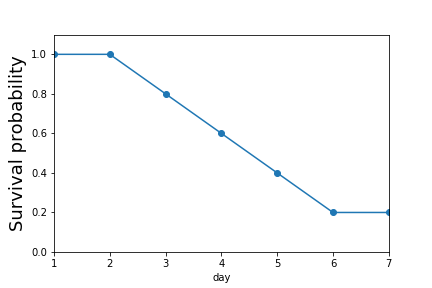
fig,ax=subplots()
_=(d.sum(axis=1)/d.shape[1]).plot(ax=ax,marker='o')
_=ax.set_ylabel('Survival probability',fontsize=18)
_=ax.axis(ymin=0,ymax=1.1)
fig.savefig('fig-statistics/survival_analysis_001.png')
#
#
#
#
#
#
#
# In[5]:
fig,axs=subplots(5,1,sharex=True,sharey=True)
fig.set_size_inches((10,6))
for i,j in enumerate(d.columns):
_=d[j].plot(ax=axs[i],marker='o')
_=axs[i].axis(ymax=1.1,ymin=-.1)
_=axs[i].set_ylabel(j)
# In[6]:
fig,ax=subplots()
_=(d.sum(axis=1)/d.shape[1]).plot(ax=ax,marker='o')
_=ax.set_ylabel('Survival probability',fontsize=18)
_=ax.axis(ymin=0,ymax=1.1)
fig.savefig('fig-statistics/survival_analysis_001.png')
#
#
#
#
# The survival probability decreases by # day.
# #
#
#
#
# There is another important recursive perspective on this
# calculation. Imagine
# there is a life raft containing $[A,B,C,D,E]$. Everyone
# survives until day two
# when \emph{A} dies. This leaves four in the life raft
# $[B,C,D,E]$. Thus, from the
# perspective of day one, the survival probability is
# the probability of surviving
# just up until day two and then surviving day two,
# $\mathbb{P}_S(t\ge 2)
# =\mathbb{P}(t\notin [0,2)\vert
# t<2)\mathbb{P}_S(t=2)=(1)(4/5)=4/5$. In words,
# this means that surviving past
# the second day is the product of surviving the
# second day itself and not having
# a death up to that point (i.e., surviving up to
# that point). Using this
# recursive approach, the survival probability for the
# third day is
# $\mathbb{P}_S(t\ge 3) =\mathbb{P}_S(t> 3)\mathbb{P}_S(t=3)=(4/5)(3/4)=3/5$.
# Recall that just before the third day, the
# life raft contains $[B,C,D,E]$ and
# on the third day we have $[B,C,E]$. Thus,
# from the perspective of just before
# the third day there are four survivors in
# the raft and on the third day there
# are three $3/4$. Using this recursive
# argument generates the same plot and comes
# in handy with censoring.
#
# ### Censoring and truncation
#
# Censoring occurs when a
# subject leaves (right censoring) or enters (left
# censoring) the study. There are
# two general types of right censoring.
# The so-called Type I right censoring is
# when a subject randomly drops
# out of the study.
# This random drop-out is another
# statistical effect that has to be accounted for
# in estimating survival. Type II
# right censoring occurs when the study is
# terminated when enough specific random
# events occur.
#
# Likewise, left censoring occurs when a subject enters the study
# prior to a certain
# date, but exactly when this happened is unknown. This happens
# in study designs
# involving two separate studies stages. For example, a subject
# might enroll in the
# first selection process but be ineligible for the second
# process. Specifically,
# suppose a study concerns drug use and certain subjects
# have used the drug before
# the study but are unable to report exactly when. These
# subjects are left
# censored. Left truncation (a.k.a. staggered entry, delayed
# entry) is similar
# except the date of entry is known. For example, a subject that
# starts taking a drug
# after being initially left out of the study.
#
# Right
# censoring is the most common so let's consider an example. Let's estimate
# the
# survival function given the following survival times in days:
#
# $$
# \{ 1, 2,3^+,4,5,6^+,7,8 \}
# $$
#
# where the censored survival times are indicated by the
# plus symbol. As before,
# the survival time at the $0^{th}$ day is $8/8=1$, the
# first day is $7/8$, the
# second day = $(7/8)(6/7)$. Now, we come to the first
# right censored entry. The
# survival time for the third day is $(7/8)(6/7)(5/5) =
# (7/8)(6/7)$. Thus, the
# subject who dropped out is not considered *dead* and
# cannot be counted as such
# but is considered just *absent* as far as the
# functional estimation of the
# probabilities goes. Continuing for the fourth day,
# we have
# $(7/8)(6/7)(5/5)(4/5)$, the fifth day, $(7/8)(6/7)(5/5)(4/5)(3/4)$, the
# sixth
# (right censored) day $(7/8)(6/7)(5/5)(4/5)(3/4)(2/2)$, and so on. We can
# summarize this in the following table:
#
# ### Hazard functions and their
# properties
#
# Generally, the *survival function* is a continuous function of time
# $S(t) =
# \mathbb{P}(T>t)$ where $T$ is the event time (e.g., time of death). Note
# that
# the cumulative density function, $F(t)=\mathbb{P}(T\le t)=1-S(t)$ and
# $f(t)=\frac{dF(t)}{dt}$ is the usual probability density function. The so-called
# *hazard function* is the instantaneous rate of failure at time $t$,
#
# $$
# h(t) = \frac{f(t)}{S(t)} = \lim_{\Delta t \rightarrow 0}\frac{\mathbb{P}(T
# \in (t,t+\Delta t]|T\ge t)}{\Delta t}
# $$
#
# Note that is a continuous-limit version of
# the calculation we performed above.
# In words, it says given the event time $T\ge
# t$ (subject has survived up to
# $t$), what is the probability of the event
# occurring in the differential
# interval $\Delta t$ for a vanishingly small
# $\Delta t$. Note that this is not
# the usual derivative-slope from calculus
# because there is no difference term in
# the numerator. The hazard function is
# also called the *force of mortality*,
# *intensity rate*, or the
# *instantaneous risk*. Informally, you can think of the
# hazard function as
# encapsulating the two issues we are most concerned about:
# deaths and the
# population at risk for those deaths. Loosely speaking, the
# probability density
# function in the numerator represents the probability of a
# death occurring in a
# small differential interval. However, we are not
# particularly interested in
# unqualified deaths, but only deaths that can happen
# to a specific at-risk
# population. Returning to our lifeboat analogy, suppose
# there are 1000 people in
# the lifeboat and the probability of anybody falling off
# the lifeboat is 1/1000.
# Two things are happening here: (1) the probability of
# the bad event is small and
# (2) there are a lot of subjects over which to spread
# the probability of that bad
# event. This means that the hazard rate for any
# particular individual is small.
# On the other hand, if there are only two
# subjects in the life raft and the
# probability of falling off is 3/4, then the
# hazard rate is high because not only
# is the unfortunate event probable, the risk
# of that unfortunate event is shared
# by only two subjects.
#
# It is a mathematical
# fact that,
#
# $$
# h(t) = \frac{-d \log S(t)}{dt}
# $$
#
# This leads to the following interpretation
#
# $$
# S(t) = \exp\left( -\int_0^t h(u)du\right) := \exp(-H(t))
# $$
#
# where $H(t)$ is the *cumulative hazard function*. Note that $H(t)=-\log S(t)$.
# Consider a subject whose survival time is 5 years. For this subject to have died
# at
# the fifth year, it had to be alive during the fourth year. Thus, the *hazard*
# at
# 5 years is the failure rate per-year, conditioned on the fact that the
# subject
# survived until the fourth year. Note that this is *not* the same as the
# unconditional failure rate per year at the fifth year, because the unconditional
# rate applies to all units at time zero and does not use information about
# survival up to that point gleaned from the other units. Thus, the *hazard
# function* can be thought of as the point-wise unconditional probability of
# experiencing the event, scaled by the fraction of survivors up to that point.
# ## Example
#
# To get a sense of this, let's consider the example where the
# probability
# density function is exponential with parameter $\lambda$,
# $f(t)=\lambda
# \exp(-t\lambda),\; \forall t>0$. This makes $S(t) = 1- F(t) =
# \exp(-t\lambda)$
# and then the hazard function becomes $h(t)=\lambda$, namely a
# constant. To see
# this, recall that the exponential distribution is the only
# continuous
# distribution that has no memory:
#
# $$
# \mathbb{P}(X\le u+t \vert X>u) = 1-\exp(-\lambda t) = \mathbb{P}(X\le t)
# $$
#
# This means no matter how long we have
# been waiting for a death to occur, the
# probability of a death from that point
# onward is the same - thus the hazard
# function is a constant.
#
#
# ### Expectations
#
# Given all these definitions, it is
# an exercise in integration by parts to show
# that the expected life remaining is
# the following:
#
# $$
# \mathbb{E}(T) = \int_0^\infty S(u) du
# $$
#
# This is equivalent to the following:
#
# $$
# \mathbb{E}(T \big\vert t=0) = \int_0^\infty S(u) du
# $$
#
# and we can likewise express the expected remaining life at $t$ as the
# following,
#
# $$
# \mathbb{E}(T \big\vert T\ge t) = \frac{\int_t^\infty S(u) du}{S(t)}
# $$
#
# ### Parametric regression models
#
# Because we are interested in how study
# parameters affect survival, we need a
# model that can accommodate regression in
# exogenous (independent) variables ($\mathbf{x}$).
#
# $$
# h(t\vert \mathbf{x})= h_o(t)\exp(\mathbf{x}^T \mathbf{\boldsymbol{\beta}})
# $$
#
# where $\boldsymbol{\beta}$ are the regression coefficients and $h_o(t)$ is the
# baseline instantaneous hazard function. Because the hazard function is always
# nonnegative, the the effects of the covariates enter through the exponential
# function. These kinds of models are called *proportional hazard rate models*.
# If
# the baseline function is a constant ($\lambda$), then this reduces to the
# *exponential regression model* given by the following:
#
# $$
# h(t\vert \mathbf{x}) = \lambda \exp(\mathbf{x}^T
# \mathbf{\boldsymbol{\beta}})
# $$
#
# ### Cox proportional hazards model
#
# The tricky part about the above proportional
# hazard rate model is the
# specification of the baseline instantaneous hazard
# function. In many cases, we
# are not so interested in the absolute hazard
# function (or its correctness), but
# rather a comparison of such hazard functions
# between two study populations. The
# Cox model emphasizes this comparison by using
# a maximum likelihood algorithm for
# a partial likelihood function. There is a lot
# to keep track of in this model, so
# let's try the mechanics first to get a feel
# for what is going on.
#
# Let $j$ denote the $j^{th}$ failure time, assuming that
# failure times are sorted
# in increasing order. The hazard function for subject
# $i$ at failure time $j$ is
# $h_i(t_j)$. Using the general proportional hazards
# model, we have
#
# $$
# h_i(t_j) = h_0(t_j)\exp(z_i \beta) := h_0(t_j)\psi_i
# $$
#
# To keep it simple, we have $z_i \in \{0,1\}$ that indicates membership in the
# experimental group ($z_{i}=1$) or the control group ($z_i=0$).
# Consider the
# first failure time, $t_1$ for subject $i$ failing is the hazard
# function
# $h_i(t_1)=h_0(t_1)\psi_{i}$. From the definitions, the probability that
# subject
# $i$ is the one who fails is the following:
#
# $$
# p_1 = \frac{h_{i}(t_1)}{\sum h_k(t_1)}= \frac{h_{0}(t_1)\psi_i}{\sum h_0(t_1)
# \psi_k}
# $$
#
# where the summation is over all surviving units up to that point. Note that the
# baseline hazard cancels out and gives the following,
#
# $$
# p_1=\frac{\psi_{i}}{\sum_k \psi_k}
# $$
#
# We can keep computing this for the other failure times to obtain
# $\{p_1,p_2,\ldots\,p_D\}$. The product of all of these is the *partial
# likelihood*, $L(\psi) = p_1\cdot p_2\cdots p_D$. The next step is to maximize
# this partial likelihood (usually logarithm of the partial likelihood) over
# $\beta$. There are a lot of numerical issues to keep track of here. Fortunately,
# the Python `lifelines`
# module can keep this all straight for us.
#
# Let's see how
# this works using the `Rossi` dataset that is available in
# lifelines.
# In[7]:
from lifelines.datasets import load_rossi
from lifelines import CoxPHFitter, KaplanMeierFitter
rossi_dataset = load_rossi()
# The Rossi dataset dataset concerns prison recidivism. The `fin` variable
# indicates whether or not the subjects received financial assistance upon
# discharge from prison.
#
# * `week`: week of first arrest after release, or
# censoring time.
#
# * `arrest`: the event indicator, equal to 1 for those arrested
# during the period of the study and 0 for those who were not arrested.
#
# * `fin`:
# a factor, with levels yes if the individual received financial aid after release
# from prison, and no if he did not; financial aid was a randomly assigned factor
# manipulated by the researchers.
#
# * `age`: in years at the time of release.
#
# *
# `race`: a factor with levels black and other.
#
# * `wexp`: a factor with levels
# yes if the individual had full-time work experience prior to incarceration and
# no if he did not.
#
# * `mar`: a factor with levels married if the individual was
# married at the time of release and not married if he was not.
#
# * `paro`: a
# factor coded yes if the individual was released on parole and no if he was not.
# * `prio`: number of prior convictions.
#
# * `educ`: education, a categorical
# variable coded numerically, with codes 2 (grade 6 or less), 3 (grades 6 through
# 9), 4 (grades 10 and 11), 5 (grade 12), or 6 (some post-secondary).
#
# * `emp1` -
# `emp52`: factors coded yes if the individual was employed in the corresponding
# week of the study and no otherwise.
# In[8]:
rossi_dataset.head()
# Now, we just have to set up the calculation in `lifelines`, using the
# `scikit-
# learn` style. The `lifelines` module handles the censoring
# issues.
# In[9]:
cph = CoxPHFitter()
cph.fit(rossi_dataset,
duration_col='week',
event_col='arrest')
cph.print_summary() # access the results using cph.summary
# The values in the summary are plotted in
# [Figure](#fig:survival_analysis_002).
#
#
#
#
#
#
#
#
#
# There is another important recursive perspective on this
# calculation. Imagine
# there is a life raft containing $[A,B,C,D,E]$. Everyone
# survives until day two
# when \emph{A} dies. This leaves four in the life raft
# $[B,C,D,E]$. Thus, from the
# perspective of day one, the survival probability is
# the probability of surviving
# just up until day two and then surviving day two,
# $\mathbb{P}_S(t\ge 2)
# =\mathbb{P}(t\notin [0,2)\vert
# t<2)\mathbb{P}_S(t=2)=(1)(4/5)=4/5$. In words,
# this means that surviving past
# the second day is the product of surviving the
# second day itself and not having
# a death up to that point (i.e., surviving up to
# that point). Using this
# recursive approach, the survival probability for the
# third day is
# $\mathbb{P}_S(t\ge 3) =\mathbb{P}_S(t> 3)\mathbb{P}_S(t=3)=(4/5)(3/4)=3/5$.
# Recall that just before the third day, the
# life raft contains $[B,C,D,E]$ and
# on the third day we have $[B,C,E]$. Thus,
# from the perspective of just before
# the third day there are four survivors in
# the raft and on the third day there
# are three $3/4$. Using this recursive
# argument generates the same plot and comes
# in handy with censoring.
#
# ### Censoring and truncation
#
# Censoring occurs when a
# subject leaves (right censoring) or enters (left
# censoring) the study. There are
# two general types of right censoring.
# The so-called Type I right censoring is
# when a subject randomly drops
# out of the study.
# This random drop-out is another
# statistical effect that has to be accounted for
# in estimating survival. Type II
# right censoring occurs when the study is
# terminated when enough specific random
# events occur.
#
# Likewise, left censoring occurs when a subject enters the study
# prior to a certain
# date, but exactly when this happened is unknown. This happens
# in study designs
# involving two separate studies stages. For example, a subject
# might enroll in the
# first selection process but be ineligible for the second
# process. Specifically,
# suppose a study concerns drug use and certain subjects
# have used the drug before
# the study but are unable to report exactly when. These
# subjects are left
# censored. Left truncation (a.k.a. staggered entry, delayed
# entry) is similar
# except the date of entry is known. For example, a subject that
# starts taking a drug
# after being initially left out of the study.
#
# Right
# censoring is the most common so let's consider an example. Let's estimate
# the
# survival function given the following survival times in days:
#
# $$
# \{ 1, 2,3^+,4,5,6^+,7,8 \}
# $$
#
# where the censored survival times are indicated by the
# plus symbol. As before,
# the survival time at the $0^{th}$ day is $8/8=1$, the
# first day is $7/8$, the
# second day = $(7/8)(6/7)$. Now, we come to the first
# right censored entry. The
# survival time for the third day is $(7/8)(6/7)(5/5) =
# (7/8)(6/7)$. Thus, the
# subject who dropped out is not considered *dead* and
# cannot be counted as such
# but is considered just *absent* as far as the
# functional estimation of the
# probabilities goes. Continuing for the fourth day,
# we have
# $(7/8)(6/7)(5/5)(4/5)$, the fifth day, $(7/8)(6/7)(5/5)(4/5)(3/4)$, the
# sixth
# (right censored) day $(7/8)(6/7)(5/5)(4/5)(3/4)(2/2)$, and so on. We can
# summarize this in the following table:
#
# ### Hazard functions and their
# properties
#
# Generally, the *survival function* is a continuous function of time
# $S(t) =
# \mathbb{P}(T>t)$ where $T$ is the event time (e.g., time of death). Note
# that
# the cumulative density function, $F(t)=\mathbb{P}(T\le t)=1-S(t)$ and
# $f(t)=\frac{dF(t)}{dt}$ is the usual probability density function. The so-called
# *hazard function* is the instantaneous rate of failure at time $t$,
#
# $$
# h(t) = \frac{f(t)}{S(t)} = \lim_{\Delta t \rightarrow 0}\frac{\mathbb{P}(T
# \in (t,t+\Delta t]|T\ge t)}{\Delta t}
# $$
#
# Note that is a continuous-limit version of
# the calculation we performed above.
# In words, it says given the event time $T\ge
# t$ (subject has survived up to
# $t$), what is the probability of the event
# occurring in the differential
# interval $\Delta t$ for a vanishingly small
# $\Delta t$. Note that this is not
# the usual derivative-slope from calculus
# because there is no difference term in
# the numerator. The hazard function is
# also called the *force of mortality*,
# *intensity rate*, or the
# *instantaneous risk*. Informally, you can think of the
# hazard function as
# encapsulating the two issues we are most concerned about:
# deaths and the
# population at risk for those deaths. Loosely speaking, the
# probability density
# function in the numerator represents the probability of a
# death occurring in a
# small differential interval. However, we are not
# particularly interested in
# unqualified deaths, but only deaths that can happen
# to a specific at-risk
# population. Returning to our lifeboat analogy, suppose
# there are 1000 people in
# the lifeboat and the probability of anybody falling off
# the lifeboat is 1/1000.
# Two things are happening here: (1) the probability of
# the bad event is small and
# (2) there are a lot of subjects over which to spread
# the probability of that bad
# event. This means that the hazard rate for any
# particular individual is small.
# On the other hand, if there are only two
# subjects in the life raft and the
# probability of falling off is 3/4, then the
# hazard rate is high because not only
# is the unfortunate event probable, the risk
# of that unfortunate event is shared
# by only two subjects.
#
# It is a mathematical
# fact that,
#
# $$
# h(t) = \frac{-d \log S(t)}{dt}
# $$
#
# This leads to the following interpretation
#
# $$
# S(t) = \exp\left( -\int_0^t h(u)du\right) := \exp(-H(t))
# $$
#
# where $H(t)$ is the *cumulative hazard function*. Note that $H(t)=-\log S(t)$.
# Consider a subject whose survival time is 5 years. For this subject to have died
# at
# the fifth year, it had to be alive during the fourth year. Thus, the *hazard*
# at
# 5 years is the failure rate per-year, conditioned on the fact that the
# subject
# survived until the fourth year. Note that this is *not* the same as the
# unconditional failure rate per year at the fifth year, because the unconditional
# rate applies to all units at time zero and does not use information about
# survival up to that point gleaned from the other units. Thus, the *hazard
# function* can be thought of as the point-wise unconditional probability of
# experiencing the event, scaled by the fraction of survivors up to that point.
# ## Example
#
# To get a sense of this, let's consider the example where the
# probability
# density function is exponential with parameter $\lambda$,
# $f(t)=\lambda
# \exp(-t\lambda),\; \forall t>0$. This makes $S(t) = 1- F(t) =
# \exp(-t\lambda)$
# and then the hazard function becomes $h(t)=\lambda$, namely a
# constant. To see
# this, recall that the exponential distribution is the only
# continuous
# distribution that has no memory:
#
# $$
# \mathbb{P}(X\le u+t \vert X>u) = 1-\exp(-\lambda t) = \mathbb{P}(X\le t)
# $$
#
# This means no matter how long we have
# been waiting for a death to occur, the
# probability of a death from that point
# onward is the same - thus the hazard
# function is a constant.
#
#
# ### Expectations
#
# Given all these definitions, it is
# an exercise in integration by parts to show
# that the expected life remaining is
# the following:
#
# $$
# \mathbb{E}(T) = \int_0^\infty S(u) du
# $$
#
# This is equivalent to the following:
#
# $$
# \mathbb{E}(T \big\vert t=0) = \int_0^\infty S(u) du
# $$
#
# and we can likewise express the expected remaining life at $t$ as the
# following,
#
# $$
# \mathbb{E}(T \big\vert T\ge t) = \frac{\int_t^\infty S(u) du}{S(t)}
# $$
#
# ### Parametric regression models
#
# Because we are interested in how study
# parameters affect survival, we need a
# model that can accommodate regression in
# exogenous (independent) variables ($\mathbf{x}$).
#
# $$
# h(t\vert \mathbf{x})= h_o(t)\exp(\mathbf{x}^T \mathbf{\boldsymbol{\beta}})
# $$
#
# where $\boldsymbol{\beta}$ are the regression coefficients and $h_o(t)$ is the
# baseline instantaneous hazard function. Because the hazard function is always
# nonnegative, the the effects of the covariates enter through the exponential
# function. These kinds of models are called *proportional hazard rate models*.
# If
# the baseline function is a constant ($\lambda$), then this reduces to the
# *exponential regression model* given by the following:
#
# $$
# h(t\vert \mathbf{x}) = \lambda \exp(\mathbf{x}^T
# \mathbf{\boldsymbol{\beta}})
# $$
#
# ### Cox proportional hazards model
#
# The tricky part about the above proportional
# hazard rate model is the
# specification of the baseline instantaneous hazard
# function. In many cases, we
# are not so interested in the absolute hazard
# function (or its correctness), but
# rather a comparison of such hazard functions
# between two study populations. The
# Cox model emphasizes this comparison by using
# a maximum likelihood algorithm for
# a partial likelihood function. There is a lot
# to keep track of in this model, so
# let's try the mechanics first to get a feel
# for what is going on.
#
# Let $j$ denote the $j^{th}$ failure time, assuming that
# failure times are sorted
# in increasing order. The hazard function for subject
# $i$ at failure time $j$ is
# $h_i(t_j)$. Using the general proportional hazards
# model, we have
#
# $$
# h_i(t_j) = h_0(t_j)\exp(z_i \beta) := h_0(t_j)\psi_i
# $$
#
# To keep it simple, we have $z_i \in \{0,1\}$ that indicates membership in the
# experimental group ($z_{i}=1$) or the control group ($z_i=0$).
# Consider the
# first failure time, $t_1$ for subject $i$ failing is the hazard
# function
# $h_i(t_1)=h_0(t_1)\psi_{i}$. From the definitions, the probability that
# subject
# $i$ is the one who fails is the following:
#
# $$
# p_1 = \frac{h_{i}(t_1)}{\sum h_k(t_1)}= \frac{h_{0}(t_1)\psi_i}{\sum h_0(t_1)
# \psi_k}
# $$
#
# where the summation is over all surviving units up to that point. Note that the
# baseline hazard cancels out and gives the following,
#
# $$
# p_1=\frac{\psi_{i}}{\sum_k \psi_k}
# $$
#
# We can keep computing this for the other failure times to obtain
# $\{p_1,p_2,\ldots\,p_D\}$. The product of all of these is the *partial
# likelihood*, $L(\psi) = p_1\cdot p_2\cdots p_D$. The next step is to maximize
# this partial likelihood (usually logarithm of the partial likelihood) over
# $\beta$. There are a lot of numerical issues to keep track of here. Fortunately,
# the Python `lifelines`
# module can keep this all straight for us.
#
# Let's see how
# this works using the `Rossi` dataset that is available in
# lifelines.
# In[7]:
from lifelines.datasets import load_rossi
from lifelines import CoxPHFitter, KaplanMeierFitter
rossi_dataset = load_rossi()
# The Rossi dataset dataset concerns prison recidivism. The `fin` variable
# indicates whether or not the subjects received financial assistance upon
# discharge from prison.
#
# * `week`: week of first arrest after release, or
# censoring time.
#
# * `arrest`: the event indicator, equal to 1 for those arrested
# during the period of the study and 0 for those who were not arrested.
#
# * `fin`:
# a factor, with levels yes if the individual received financial aid after release
# from prison, and no if he did not; financial aid was a randomly assigned factor
# manipulated by the researchers.
#
# * `age`: in years at the time of release.
#
# *
# `race`: a factor with levels black and other.
#
# * `wexp`: a factor with levels
# yes if the individual had full-time work experience prior to incarceration and
# no if he did not.
#
# * `mar`: a factor with levels married if the individual was
# married at the time of release and not married if he was not.
#
# * `paro`: a
# factor coded yes if the individual was released on parole and no if he was not.
# * `prio`: number of prior convictions.
#
# * `educ`: education, a categorical
# variable coded numerically, with codes 2 (grade 6 or less), 3 (grades 6 through
# 9), 4 (grades 10 and 11), 5 (grade 12), or 6 (some post-secondary).
#
# * `emp1` -
# `emp52`: factors coded yes if the individual was employed in the corresponding
# week of the study and no otherwise.
# In[8]:
rossi_dataset.head()
# Now, we just have to set up the calculation in `lifelines`, using the
# `scikit-
# learn` style. The `lifelines` module handles the censoring
# issues.
# In[9]:
cph = CoxPHFitter()
cph.fit(rossi_dataset,
duration_col='week',
event_col='arrest')
cph.print_summary() # access the results using cph.summary
# The values in the summary are plotted in
# [Figure](#fig:survival_analysis_002).
#
#
#
#
# This shows the fitted coefficients # from the summary table for each covariate.
# #
#
# In[10]:
ax=cph.plot();
ax.figure.savefig('fig-statistics/survival_analysis_002.png')
# The Cox proportional hazards model object from `lifelines` allows us to predict
# the survival function for an individual with given covariates, assuming that
# the
# individual just entered the study. For example, for the first individual
# (i.e.,
# row) in the `rossi_dataset`, we can use the model to predict the
# survival
# function for that individual.
# In[11]:
cph.predict_survival_function(rossi_dataset.iloc[0,:]).head()
# This result is plotted in [Figure](#fig:survival_analysis_003).
# In[12]:
fig,ax =subplots()
_=cph.predict_survival_function(rossi_dataset.iloc[0,:]).plot(ax=ax)
_=ax.set_ylabel('Survival probability',fontsize=16)
_=ax.set_title('Survival probability for $0^{th}$ subject',fontsize=18)
fig.savefig('fig-statistics/survival_analysis_003.png')
#
#
#
#
#
#
#
#
#
#
#
#
#
#
#
#
#
#
#
#
#
#
# In[10]:
ax=cph.plot();
ax.figure.savefig('fig-statistics/survival_analysis_002.png')
# The Cox proportional hazards model object from `lifelines` allows us to predict
# the survival function for an individual with given covariates, assuming that
# the
# individual just entered the study. For example, for the first individual
# (i.e.,
# row) in the `rossi_dataset`, we can use the model to predict the
# survival
# function for that individual.
# In[11]:
cph.predict_survival_function(rossi_dataset.iloc[0,:]).head()
# This result is plotted in [Figure](#fig:survival_analysis_003).
# In[12]:
fig,ax =subplots()
_=cph.predict_survival_function(rossi_dataset.iloc[0,:]).plot(ax=ax)
_=ax.set_ylabel('Survival probability',fontsize=16)
_=ax.set_title('Survival probability for $0^{th}$ subject',fontsize=18)
fig.savefig('fig-statistics/survival_analysis_003.png')
#
#
#
#
#
#
#
#
#
#
#
#
#
#
#
#
#
#
#
# The Cox # proportional hazards model can predict the survival probability for an # individual based on their covariates.
# #
#
# In[ ]:
#
#
# In[ ]: